
Elasticsearch does an awesome job when it comes to working with maps. providing several ways of visualizing your data. But ever since I started working on the Elasticsearch integration, I’ve wanted to display Pokémon encounters on a map. Although I couldn’t do it exactly as I wanted, turns out that it is not that hard to use your custom maps.
We will be picking off from where we stopped in the previous article. The complete code can be found in this repository on GitHub.
Creating a Kanto region map file
The first thing we need to do is to create a GeoTIFF (GTiff) file. This can be done using the GDAL library, used for raster and vector geospatial data formats. So grab your favorite Kanto map (I chose to take a print screen of the in-game map) and run the following commands. Do pay attention to the name parameter, in case you didn’t name it “kanto_map.png” as I did.
gdal_translate -of GTiff -a_srs EPSG:4326 -a_ullr -105 45 105 -45 kanto_map.png kanto_map_gtiff.tiff
gdal_warp -t_srs EPSG:4326 kanto_map_gtiff.tiff kanto_map.tiff
Setting up GeoServer
If we want to use a different map in Kibana besides the base one, it needs to come from somewhere. An option is to use GeoServer, which implements the Web Map Service (WMS) format. GeoServer is a server that allows users to view and edit geospatial data, that supports multiple open standards.
Creating the GeoServer docker image
We will be using Docker to run our GeoServer, since it makes things so much easier for us. The updates are going to be based on this docker image, only removing some unnecessary stuff for our case. These are going to be the new additions:
Creating a datastore
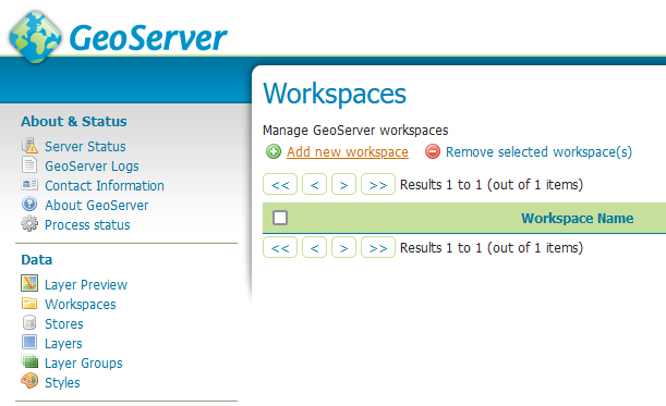
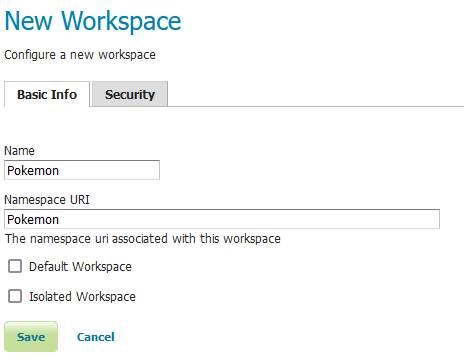
With our containers running, we will begin by creating a new workspace. Navigate to Data > Workspaces, then click on “Add a new workspace. In this case, we will set both the Name and the Namespace URI to “Pokemon”.
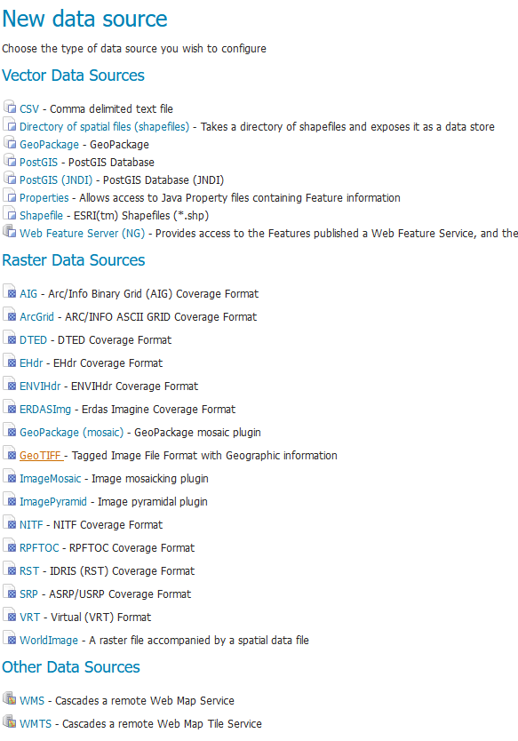
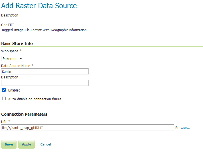
Once that’s done, we need to create the Data Store. So navigate to Data > Stores and click on “Add new store”. Choose “GeoTIFF” from the list of data sources. In the next screen, we are going to name it “Kanto”, and then in the URL field, browse to the GeoTIFF file we created earlier.
You might have to copy the file to your container, which can be done by using docker cp. You can find an example below. It copies the local file “kanto_map_gtiff.tiff” to the root folder of the container with ID 8bd4c8b9747c.
docker cp .\kanto_map_gtiff.tiff 8bd4c8b9747c:/Once you are done, press “Save”. In the next screen, simply click on “Publish” and press “Save” again. And that’s it! Your map is ready to be served. If you wanna preview it, you can navigate to Data > Layer Preview and choose a format, such as OpenLayers.
Adding the map visualization in Kibana
With the GeoServer up and running, we can now create a new map visualization in Kibana that consumes it. Browse to your Kibana deployment (usually http://localhost:5601/), then in the side menu navigate to Analytics > Visualize Library. Press “Create new visualization” and choose “Maps”.
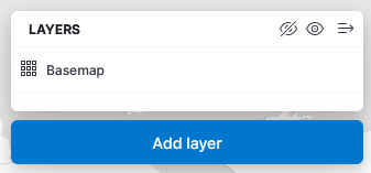
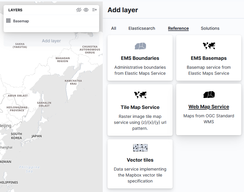
You should now have the default map visualization on your screen. Press the “Add layer” button, located in the upper right corner, and choose “Web Map Service”. We will need to provide the URL for our WMS, which is http://localhost:8600/geoserver/Pokemon/wms in this case. Click “Load capabilities” and it should display some extra fields. Select “kanto_map_gtiff” in the Layers field and click “Add Layer”.
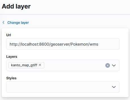
We now have the Kanto region map displayed on our screen, awesome! But before we can actually see our data here, we need to update our index to include some location data.
Adding a GeoLocation field to the index
The first thing we are going to do is to create a new struct called “PokemonLocation”, which will contain the name of a map and its GeoLocation. You might be wondering why the GeoLocation is null, but don’t worry, you’ll understand why very soon.
Once created, we can use it in our PokemonInformation struct. We are now receiving the PokemonLocation in the constructor, simply using its properties to initialize the PokemonInformation struct. Notice that we are also adding a property called Number. The reason is that later, in our map, we will only show a single icon per Pokemon, not one for every encounter, and using a number instead of a string makes our comparison faster.
In our Bootstrapper class, the change is minimal as well. When creating the PokemonInformation struct, we are now providing a PokemonLocation struct and the number of the Pokémon.
There’s not much mystery to the PokemonNameToNumberConverter class either, it just maps from a string to a number. We had to resort to this converter, as I could not find which memory address holds the value for the foe’s Pokemon number.
For the creation of PokemonLocation structs, I decided to move it to a Factory class to better organize my code. The Bootstrapper class is already a bit messy, so let’s not make it worse. The only catch in this class is the tiny scrambling that happens in the location. The ByteToLatLonGeoLocationConverter returns us the exact position in the map for the route the player was in, but if we were to use it as is, all Pokémon dots would appear in the exact same space in the map.
Lastly, the ByteToLatLonGeoLocationConverter class receives the ID of the map that the Pokémon was caught and returns the coordinates. The problem here is that those coordinates must be found manually. For example, for Route 22 I hovered my mouse approximately at the center of where it is in the map, then wrote down the coordinates. And since these coordinates depend on how the map was generated, another person following these steps might get different results than I did. So for my small test, I only tried a single Route. And that’s why we have a nullable PokemonLocation struct in our PokemonInformation struct.
Notice that if this isn’t your first time running this solution, your index changes won’t make it to Elasticsearch, since the solution doesn’t support updating the mapping of an index. To work around that, you can either add the mapping manually, or delete the index through Kibana.
Displaying Pokémon encounters on the map
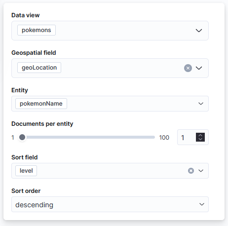
Now that we are including the coordinates in our index, we can update our existing visualization to display the data we want. Let’s begin by adding another layer of type “Top hits per entity”. In that screen, you will have the following fields:
- Geospatial field: the field that contains the location data, which is the one we just added.
- Entity: the field that identifies entities in the documents, used to aggregate them into buckets. For us, it’s the pokemonName.
- Documents per entity: How many documents we wanna display in this layer. One is enough for us.
- Sort field: the field used to sort the documents, to define what’s the top document. It doesn’t really matter for us, but we are going for level.
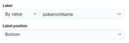
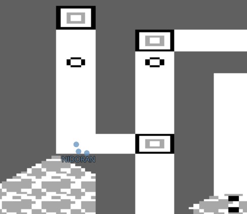
Click on “Add layer” and you should start seeing some dots in your maps now. Unfortunately, that doesn’t really help us easily see which Pokémon are found in each route, right? We can improve it a bit by adding captions to it. Edit your layer, search for the Layer Style category, and set the “pokemonName” to the “Label field”. That gives us a small improvement, but it’s not really useful for cases where the dots are so close to each other, which is precisely our case.
Another option to improve the visualization would be to use custom icons instead of simple dots, which has two problems. The first one is that we would need to manually add and map the icons to each Pokémon, and that would be a bit tiring. I suppose that one way to solve the mapping part would be to export the visualization, edit the generated file, and import it again. I haven’t tried that because of two reasons: I couldn’t find a way to import 151 SVGs files besides doing it manually, and because of the second issue I mentioned earlier.
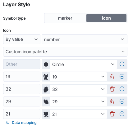
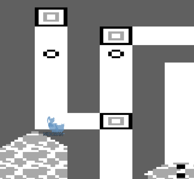
The second issue is that Elasticsearch doesn’t really expect us to provide beautiful and colored SVGs, it’s expecting an icon. So as you can see in the image above, they lose their original colors and are added like shadows, as the color is supposed to come from the “Fill color” field. In the end, it feels like we are playing “Who’s that Pokémon?”.
Conclusion
It was really simple to set up GeoServer and add the Kanto region map to Kibana, all thanks to this article from Jay Greenberg. But when it came to displaying the data, things didn’t go as planned. Hopefully, in the future, a customer will come up with a legitimate use case where they need to have hundreds of images in a map, so this can be concluded the way it was intended to.